Let's be optimistic and assume we have designed a sound experiment. Can anything else can go wrong? Unfortunately, yes: the data-collection procedure can introduce spurious effects called sampling biases. Imagine the following confession of an elementary school mathematics teacher: ``I have resisted this conclusion for years, but I really don't think girls are good at mathematics. They rarely ask good questions and they rarely give good answers to the questions I ask.'' This confession disturbs you, so you ask to see a class for yourself. And what you find is that the teacher rarely calls on the girls. This is a sampling bias. The procedure for collecting data is biased against a particular result, namely, girls asking or answering questions well.
We encountered a subtle sampling bias in an experiment with the Phoenix system. The first hint of trouble was an obviously incorrect result, namely, wind speed and finish time were uncorrelated. We knew that higher wind speeds caused the fire to spread faster, which required more fireline to be cut, which took more time; so obviously wind speed and finish time ought to be positively correlated. But our data set included only successfully-contained fires, and we defined success to mean a fire is contained in 150 simulated hours or less. Suppose the probability of containing an ``old'' fire--one that isn't contained relatively quickly--by the 150-hour cutoff, is small, and this probability is inversely proportional to wind speed. Then at higher wind speeds, fewer old fires will be successfully contained, so the sample of successfully-contained fires will include relatively few old fires fought at high wind speeds, but plenty of old fires fought at low wind speeds. Figure 3.6 is a schematic illustration of this situation (our sample contained 215 fires instead of the 27 illustrated). Relatively few fires are contained at high wind speeds, and only one of these burned for more than 100 hours. In contrast, many fires are contained at low wind speeds and four of these burned for more than 100 hours. Clearly, old fires are under-represented at high wind speeds. Two opposing effects--the tendency to contain fires earlier at low wind speeds, and the under-representation of old fires at high wind speeds--cancel out, yielding a correlation between wind speed and finish time of approximately zero (r = .006). Note, however, that one of these effects is legitimate and the other is spurious. The positive relationship between wind speed and finish time is legitimate; the negative relationship is due entirely to sampling bias.
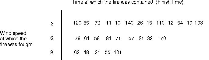
Figure 3.6 An illustration of sampling bias.
The genesis of the sampling bias was the decision to include in our sample only fires that were contained by a particular cut-off time. Whenever a cut-off time determines membership in a sample, the possibility of sampling bias arises, and it is certain if time and the independent variable interact to affect the probability that a trial will finish by the cut-off time. It takes longer to contain fires at high wind speeds, so the independent variable (wind speed) has a simple effect on the probability that a trial will be included in a sample. But in addition, the effect of wind speed on this probability changes over time. As time passes, the probability of completing a trial decreases at different rates determined by wind speed. Because this interaction between wind speed and time affects the probability of completing a trial by the cut-off time, it is, by definition, a sampling bias.
It would help to have a way to detect sampling biases when they occur. A clue can often be found in frequency distributions of the dependent variable, y, at different levels of the independent variable, x. Before we show an example, let's consider a model of the effects of the independent variable. It is commonly assumed that x changes the location of the distribution of y but not its shape. This is illustrated schematically in Figure 3.7. The effect of increasing values of x is to shift the mean of y, but not to change the shape of y's distribution. But what if changing x also changed the shape of this distribution, as shown in Figure 3.8? The problem isn't only that the x = 1 curve includes fewer data points; this could be explained by x = 1 comprising a more difficult set of problems than x = 2, and is not a sampling bias. The problem is that the x = 1 curve is not symmetric while the x = 2 curve is. This means that whereas x = 2 yields high and low scores in equal proportion, medium-to-high scores are disproportionately rare when x = 1. If x = 1 problems are simply more difficult than x = 2 problems, we would still expect to see medium-to-high and low scores in equal proportion. Instead, it appears that x affects not only the score but also the probability of a relatively high score. This suggests the presence of another factor that influences membership in the sample and is itself influenced by x, in other words, a sampling bias.
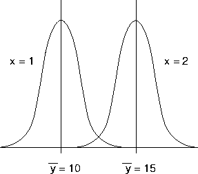
Figure 3.7 An effect of x changes the location of a distribution.
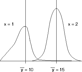
Figure 3.8An effect of x changes the location and shape of a distribution.
Let us see whether the frequency histograms of finish time at different levels of WindSpeed disclose a sampling bias, as the previous discussion suggests. In Figure 3.9, which shows the distributions, we see immediately that the slow WindSpeed distribution has a shape very different than the others. Each distribution has a big mode in the 10-40 range, but the medium and fast WindSpeed distributions are pretty flat beyond their modes, whereas the slow WindSpeed distribution is bimodal. We expected WindSpeed to affect the locations of these distributions (in fact, the modal finish times are 10, 20 and 25 for slow, medium and fast, respectively), but why should WindSpeed affect the shapes of the distributions? Well, as we know, WindSpeed speed interacts with time to affect the probability that a trial will be included in the sample. Thus, frequency distributions of a dependent variable at different levels of the independent variable suggest a sampling bias, if, as in Figure 3.9, they have different shapes.
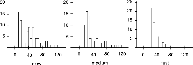
Figure 3.9 Distributions of finish times for three wind speeds, illustrating a sampling bias.