A dependent variable represents, more or less faithfully, aspects of the behavior of a system. Often the dependent variable is a measure of performance such as hit rate or run time or mean time between failures. Some dependent variables are better than others. In general, continuous dependent variables such as time are preferable to categorical variables such as success or ordinal variables such as letter grades. It is easier to discern a functional relationship between x and y if values of x map to a continuous range of y values instead of discrete bins. Other criteria are: dependent variables should be easy to measure; they should be relatively insensitive to exogenous variables (i.e., their distributions should have low standard deviations); and they should measure what you intend them to measure.
The latter criterion sounds trite, but remember, variables are representations and they can easily be misrepresentations (see section 2.1.3). Consider this simple but still unresolved design question. Adele Howe added a failure recovery component to the Phoenix planner which allowed it to get out of trouble by changing its plans dynamically. She implemented several failure recovery methods. The obvious question is, which methods are best? If some accomplish more than others with comparable costs, then, clearly, they are better. Now, the only question is, how should the benefits of a failure recovery method be measured? The answer is not obvious. To illustrate the difficulty, look at the ``timeline'' representation of failure recovery in Figure 3.10. A good failure recovery method should fix a plan quickly (i.e., C should be small) and should modify the plan in such a way that it runs for a long time before the next failure (i.e., D should be large). C and D, then, are measures of the costs and benefits, respectively, of failure recovery.
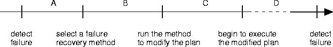
Figure 3.10 A timeline representation of failure recovery.
Unfortunately, plans can run for long periods making little progress but not failing, either; so large values of D are not always preferred. In fact, we prefer small values of D if the modified plan makes little progress. A good method, then, modifies a plan so it either runs for a long time before the next failure and makes a lot of progress, or fails quickly when it would probably not make much progress. The trouble is we cannot assess the latter condition--we cannot say whether a failed plan might have progressed. Thus we cannot say whether a plan modification is beneficial when the modified plan fails quickly.
In rare instances one can analyze mathematically whether a dependent variable actually represents the aspects of behavior it is supposed to represent. A good example is due to Fayyad and Irani Fayyad (1990), who asked, ``What is a good measure of the quality of decision trees induced by machine learning algorithms?'' Decision trees are rules for classifying things; for example, Figure 3.11 shows a fragment of a tree for classifying animals. Decision trees (and the algorithms that generate them) are usually evaluated empirically by their classification accuracy on test sets. For example, the tree in Figure 3.11 would incorrectly classify a penguin as a turtle, and so would achieve a lower classification accuracy score than a tree that classified penguins as birds (all other things being equal). Fayyad and Irani invented a method to judge whether an algorithm is likely to generate trees with high classification accuracy, without actually running lots of test cases. They proved that the number of leaves in a decision tree is a proxy for several common performance measures; in particular, trees with fewer leaves are likely to have higher classification accuracy than leafier trees:
Suppose one gives a new algorithm for generating decision trees, how then can one go about establishing that it is indeed an improvement? To date, the answer...has been: Compare the performance of the new algorithm with that of the old algorithm by running both on many data sets. This is a slow process that does not necessarily produce conclusive results. On the other hand, suppose one were able to prove that given a data set, Algorithm A will always (or `most of the time') generate a tree that has fewer leaves than the tree generated by Algorithm B. Then the results of this paper can be used to claim that Algorithm A is `better' than Algorithm B. (Fayyad 1990, p.754),
Thus, Fayyad and Irani demonstrate that we sometimes can find a formal basis for the claim that one dependent variable is equivalent to (or, in this case, probabilistically indicative of) another.
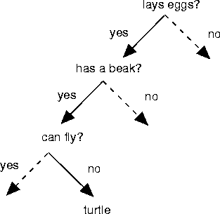
Figure 3.11 A small fragment of a decision tree for classifying animals.