P300 Waves for Single Subjects
The Stimulus Channel
Each data file includes EEG recorded during a visual stimulus protocol designed to elicit P300 waves. In the single-letter protocol, subjects looked at a computer screen in the center of which single letters were briefly displayed sequentially, in a random order. In the first trial, they were asked to count the number of times the letter ‘b’ appeared. They were then asked to count the number of times the letter ‘d’ appeared, and then again counting the number of times the letter ‘p’ appeared. These three trials were then repeated, but instead of displaying a single letter, nine letters were simultaneously displayed, in a three-by-three table. Subjects were asked to count the number of times the letter ‘b’ appeared in the center of the table, and similarly the letter ‘d’, and the letter ‘p’.
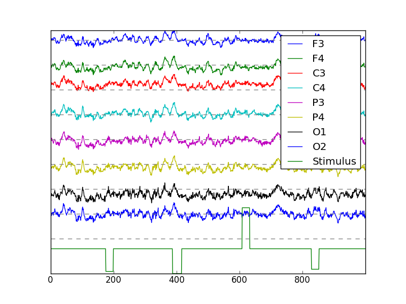
The letter being presented in the center of the computer screen is indicated in the stimulus channel of the data. For the g.tec g.GAMMAsys data files, this is the ninth channel. We can see this by again plotting all nine channels, but this time of the seventh element (index 6) in the data list, the one for which the protocol is letter-b.
In [1]: import json

In [2]: import numpy as np

In [3]: import matplotlib.pyplot as plt

In [4]: data = json.load(open('s21-gammasys-gifford-unimpaired.json','r'))

In [5]: letterd = data[4]

In [6]: letterd['protocol']
Out[6]: u'letter-d'

# Note the transpose here.  Time now advances by row.  Columns are channels
In [7]: eeg = np.array(letterd['eeg']['trial 1']).T

In [8]: plt.ion()

In [9]: plt.figure();

In [10]: plt.plot(eeg[4000:5000,:9] + 80*np.arange(8,-1,-1));

In [11]: plt.plot(np.zeros((1000,9)) + 80*np.arange(8,-1,-1),'--',color='gray');

In [12]: plt.yticks([]);

In [13]: plt.legend(letterd['channels'] + ['Stimulus']);

In [14]: plt.axis('tight');
The stimulus channel has the values
In [1]: np.unique(eeg[:,8])
Out[1]:
array([-118., -116., -115., -112., -110., -109., -107., -105., -102.,
       -101.,  -98.,  -97.,  -32.,    0.,  100.])
Its value is 0 only before the trial starts. Of the non-zero values, only one is positive. This represents the letter to be counted—the target letter. The negative values are nontarget letters, except for -32, which is the ASCII code for a blank representing the times when no letter is displayed and the computer screen is black. The ASCII codes for all stimulus channel values can be converted to letters by
In [1]: [chr(int(n)) for n in np.abs(np.unique(eeg[:,8]))]
Out[1]: ['v', 't', 's', 'p', 'n', 'm', 'k', 'i', 'f', 'e', 'b', 'a', ' ', '\x00', 'd']
Segmenting Data into Time Windows
To investigate the presence or absence of P300 waves, we must segment the data into time windows following each stimulus presentation. First, let’s take a closer look. Plot just the data from the stimulus channel (index 8) and Channel P3 (index 5).
In [1]: plt.clf();

In [2]: plt.plot(eeg[3000:4500,[5,8]]);

In [3]: plt.axis('tight');

In [4]: plt.xlabel('Time Samples');
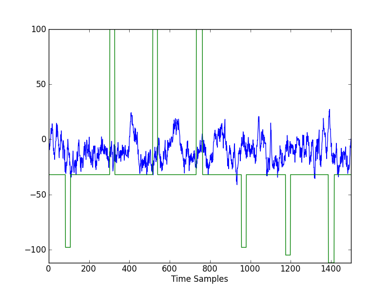
It appears that some P300 waves are present following the three positive stimuli. Remember that this is the target letter ‘d’. The positive wave appears roughly 100 samples after the stimulus onset. Since the sampling frequency is 256 Hz, this is about 0.4 seconds, or 400 milliseconds, after the stimulus.
In [1]: 100.0 / letterd['sample rate']
Out[1]: 0.390625
Now let’s collect all of the segments from this letter ‘d’ trial. First, find the sample indices where each stimulus starts, collect the displayed letters for each stimulus, and keep track of which stimuli are the target letter.
In [1]: starts = np.where(np.diff(np.abs(eeg[:,-1])) > 0)[0]

In [2]: stimuli = [chr(int(n)) for n in np.abs(eeg[starts+1,-1])]

In [3]: targetLetter = letterd['protocol'][-1]

In [4]: targetSegments = np.array(stimuli) == targetLetter

In [5]: len(starts),len(stimuli),len(targetSegments)
Out[5]: (80, 80, 80)

In [6]: for i,(s,stim,targ) in enumerate(zip(starts,stimuli,targetSegments)):
   ...:      print s,stim,targ,'; ',
   ...:      if (i+1) % 5 == 0:
   ...:          print
   ...:
247 b False ;  465 a False ;  683 p False ;  899 d True ;  1119 p False ;
1337 b False ;  1551 p False ;  1771 d True ;  1985 b False ;  2207 b False ;
2427 n False ;  2643 v False ;  2863 d True ;  3082 b False ;  3302 d True ;
3515 d True ;  3731 d True ;  3955 b False ;  4174 i False ;  4386 p False ;
4607 d True ;  4827 b False ;  5043 b False ;  5262 a False ;  5482 p False ;
5695 p False ;  5919 d True ;  6135 d True ;  6351 d True ;  6567 b False ;
6787 t False ;  7007 b False ;  7223 d True ;  7443 d True ;  7659 t False ;
7879 d True ;  8095 p False ;  8317 p False ;  8533 s False ;  8749 p False ;
8971 b False ;  9187 d True ;  9402 p False ;  9626 s False ;  9843 b False ;
10059 m False ;  10275 i False ;  10495 m False ;  10711 p False ;  10930 p False ;
11147 p False ;  11367 b False ;  11583 d True ;  11805 k False ;  12023 p False ;
12235 p False ;  12458 p False ;  12679 b False ;  12893 d True ;  13109 d True ;
13333 v False ;  13551 f False ;  13770 n False ;  13987 d True ;  14202 f False ;
14418 e False ;  14635 k False ;  14855 b False ;  15075 p False ;  15290 b False ;
15514 p False ;  15731 p False ;  15945 b False ;  16162 p False ;  16382 d True ;
16599 d True ;  16818 b False ;  17042 e False ;  17258 b False ;  17475 b False ;
Good. Now, how long should each time window be? The number of samples between each stimulus onset is
In [1]: np.diff(starts)
Out[1]:
array([218, 218, 216, 220, 218, 214, 220, 214, 222, 220, 216, 220, 219,
       220, 213, 216, 224, 219, 212, 221, 220, 216, 219, 220, 213, 224,
       216, 216, 216, 220, 220, 216, 220, 216, 220, 216, 222, 216, 216,
       222, 216, 215, 224, 217, 216, 216, 220, 216, 219, 217, 220, 216,
       222, 218, 212, 223, 221, 214, 216, 224, 218, 219, 217, 215, 216,
       217, 220, 220, 215, 224, 217, 214, 217, 220, 217, 219, 224, 216, 217])
and the minimum number is
In [1]: np.min(np.diff(starts))
Out[1]: 212
so let’s use time windows of 210 samples. We can build a matrix with rows being segments, and each row being all indices for that segment by doing this.
In [1]: indices = np.array([ np.arange(s,s+210) for s in starts ])

In [2]: indices.shape
Out[2]: (80, 210)
And, finally, we can build an 80 x 210 x 8 array of segments.
In [1]: segments = eeg[indices,:8]

In [2]: segments.shape
Out[2]: (80, 210, 8)
Grand Averages to Show P300 Waves
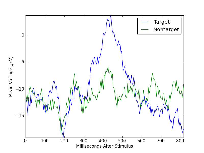
Typically, segments are averaged to minimize the effect of variations across multiple stimuli and, hopefully, to emphasize the parts of the signal that are common to the stimuli. Let’s average all of the target segments and all of the nontarget segments for the P4 channel (index 5), and plot two resulting mean segments.
In [1]: segments[targetSegments,:,5].shape
Out[1]: (20, 210)

In [2]: targetMean = np.mean(segments[targetSegments,:,5],axis=0)

In [3]: nontargetMean = np.mean(segments[targetSegments==False,:,5],axis=0)

In [4]: plt.clf();

In [5]: xs = np.arange(len(targetMean)) / 256.0 * 1000  # milliseconds

In [6]: plt.plot(xs, np.vstack((targetMean,nontargetMean)).T);

In [7]: plt.legend(('Target','Nontarget'));

In [8]: plt.axis('tight');

In [9]: plt.xlabel('Milliseconds After Stimulus');

In [10]: plt.ylabel('Mean Voltage ($\mu$ V)');

Remember that the target mean is over 20 segments, while the nontarget mean is over 60 segments. If we balance these numbers by randomly selecting 20 nontarget segments, the means look like
In [1]: targetMean = np.mean(segments[targetSegments,:,5],axis=0)

In [2]: nontargetSegments = segments[targetSegments==False,:,5]

In [3]: selectThese = np.random.permutation(range(nontargetSegments.shape[0]))[:20]

In [4]: nontargetMean = np.mean(nontargetSegments[selectThese,:],axis=0)

In [5]: plt.clf();

In [6]: plt.plot(xs, np.vstack((targetMean,nontargetMean)).T);

In [7]: plt.legend(('Target','Nontarget'));

In [8]: plt.axis('tight');

In [9]: plt.xlabel('Milliseconds After Stimulus');

In [10]: plt.ylabel('Mean Voltage ($\mu$ V)');
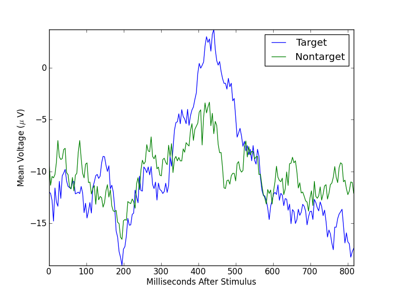
Running the above code again, with a different random selection of nontarget trials, results in a different nontarget mean.